How to draw NACA 6-Series Airfoils?

Question

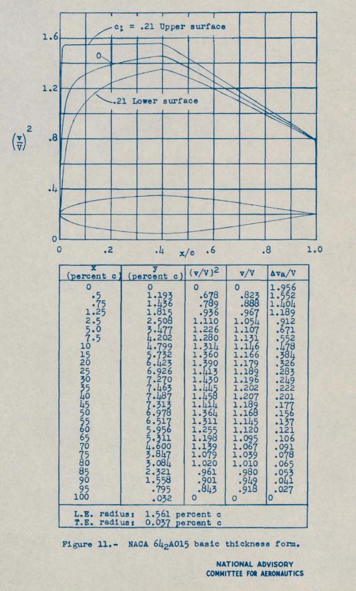
In relation to the question on the NACA 64-2A015 airfoil I would like to know how to draw this airfoil.

At least these two reports [1,2] by NASA provide the equation for it.

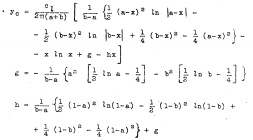
However, I am not able to find the correct parameters to draw it, so that it would match up with the coordinates given in the table above.

Here is the Matlab code I used:

a = 0.4;
b = 1.0; % caution for NON-unity entries change the equation for h
% c = 1; to simplifiy the equation the chord is set to 1

cl = 1;

g = -1/(b-a) * (a^2 * (1/2  * log(a) -1/4) - b^2 * (1/2 * log(b) -1/4)); % g  = -1/(1-a) * (a^2 * (1/2 * log(a) -1/4) + 1/4)
h = 1/(1-a) * (1/2*(1-a)^2 * log(1-a) -1/4*(1-a)^2)+g; % simplified version for b = 1: h =  1/(b-a) * (1/2*(1-a)^2 * log(1-a) - 1/2 * (1-b)^2 * log(1-b) + 1/4*(1-b)^2 - 1/4*(1-a)^2) + g

x = (0:0.001:1);
y  = cl/(2*pi*(a+b)) * ( 1/(b-a) .* (1/2 * (a-x).^2 .* log(abs(a-x)) - 1/2 .* (b-x).^2 .* log(abs(b-x)) + 1/4 .* (b-x).^2 - 1/4 .* (a-x).^2) - x.*log(x) + g - h.*x); % y = cl/(2*pi*(a+1)) * ( 1/(1-a) .* (1/2 * (a-x).^2 .* log(abs(a-x)) - 1/2 .* (1-x).^2 .* log(abs(1-x)) + 1/4 .* (1-x).^2 + 1/4 .* (a-x).^2) - x.*log(x) + g - h.*x);

L6j01_x = [0, 0.005, 0.0075, 0.0125, 0.025, 0.05, 0.075, 0.1, 0.15, 0.2, 0.25, 0.3, 0.35, 0.4, 0.45, 0.5, 0.55, 0.6, 0.65, 0.7, 0.75, 0.8, 0.85, 0.9, 0.95, 1];
L6j01_y = [0, 0.01193, 0.01436, 0.01815, 0.02508, 0.03477, 0.04202, 0.04799, 0.05732, 0.06423, 0.06926, 0.0727, 0.07463, 0.07487, 0.07313, 0.06978, 0.06517, 0.05956, 0.05311, 0.046, 0.03847, 0.03084, 0.02321, 0.01558, 0.00795, 0.00032];

plot(x,y), axis equal, hold on
plot(L6j01_x, L6j01_y,'ro'), hold off

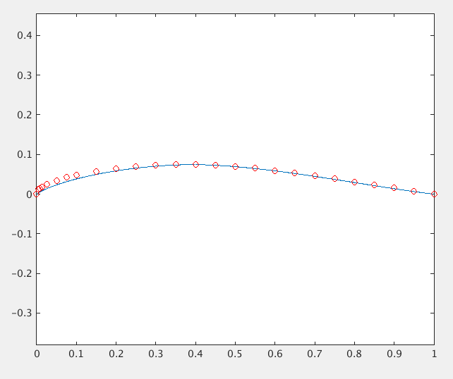
It seems my Leading Edge definition is not right. Any suggestions on how to adjust the front part of the airfoil-section?

Answer 1

From this reference:

$$c_f=K_1\cdot \frac {t}{c} + K_2(\frac {t}{c})^2 + K_3(\frac {t}{c})^3 + K_4(\frac {t}{c})^4$$

For the 64A series:

• $K_1$ = 8.2125018
• $K_2$ = 0.7685596
• $K_3$ = 1.4922345
• $K_4$ = 3.6130133

$c_f$ is the particular scale factor for this profile. And then the reference continues with this head spinning further explanation:

Now, for a specified family and thickness, the thickness distribution may be determined without iteration. From the thickness, the scale factor is computed from the polynomial function shown above. Then, the scale factor is used to multiply the basic values of the psi and epsilon functions for this airfoil family. These scaled psi and epsilon functions are used in mapping the z-plane to the z'-plane shown in Figure 1. The Joukowski function zeta = z' + 1/z' then maps the z'-plane into the zeta-plane and these results are normalized so that the leading edge is at x=0 and the trailing edge is at x=1.

Hope this helps, my head hurts after reading that.

Answer 2

The 1- and 6-series airfoils were the first which used a target pressure distribution to define the contour of the surface. This was a major progress in airfoil design but makes it impossible to use a simple equation to exactly describe the contour mathematically. The older, 4-digit series simply used the mean of a collection of successful early airfoils.

I have always used a collection of Fortran subroutines to generate the contour, and it uses tabulated data and splines to generate the shape. Here is a link to a similar collection, but in all cases you will only get an approximation. Use XFOIL or similar code to refine the pressure distribution as desired.

Answer 3

What do you mean that the chart fails to give the leading edge (LE) radius? It plainly states that the leading edge radius is 1.561% of the chord. Let's just call the chord the unit of "1" to make things easier. Anything larger or smaller is simply a ratio, right? Therefore, the LE radius is 1.561 The plot looks to be symmetrical, mirrored across the chord line. Maybe I am reading too much into this. Regardless, I hope this helps. Other airfoils generally give the upper and lower coordinates, that's why I surmise the plot is symmetrical across the chord line.